F-distribution

In probability theory and statistics, the F-distribution or F-ratio, also known as Snedecor's F distribution or the Fisher–Snedecor distribution (after Ronald Fisher and George W. Snedecor), is a continuous probability distribution that arises frequently as the null distribution of a test statistic, most notably in the analysis of variance (ANOVA) and other F-tests.

Definitions

The F-distribution with d₁ and d₂ degrees of freedom is the distribution of

${\displaystyle X={\frac {U_{1}/d_{1}}{U_{2}/d_{2}}}}$

where ${\textstyle U_{1}}$ and ${\textstyle U_{2}}$ are independent random variables with chi-square distributions with respective degrees of freedom ${\textstyle d_{1}}$ and ${\textstyle d_{2}}$.

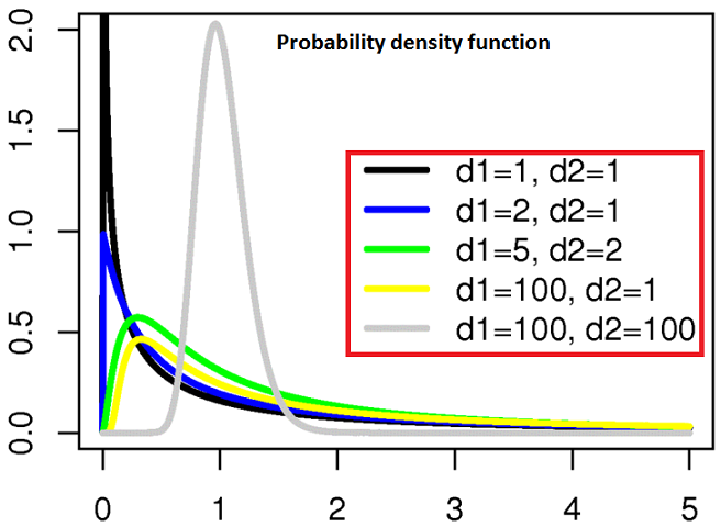
It can be shown to follow that the probability density function (pdf) for X is given by

${\displaystyle {\begin{aligned}f(x;d_{1},d_{2})&={\frac {\sqrt {\frac {(d_{1}x)^{d_{1}}\,\,d_{2}^{d_{2}}}{(d_{1}x d_{2})^{d_{1} d_{2}}}}}{x\operatorname {B} \left({\frac {d_{1}}{2}},{\frac {d_{2}}{2}}\right)}}\\[5pt]&={\frac {1}{\operatorname {B} \left({\frac {d_{1}}{2}},{\frac {d_{2}}{2}}\right)}}\left({\frac {d_{1}}{d_{2}}}\right)^{\frac {d_{1}}{2}}x^{{\frac {d_{1}}{2}}-1}\left(1 {\frac {d_{1}}{d_{2}}}\,x\right)^{-{\frac {d_{1} d_{2}}{2}}}\end{aligned}}}$

for real x > 0. Here ${\displaystyle \mathrm {B} }$ is the beta function. In many applications, the parameters d₁ and d₂ are positive integers, but the distribution is well-defined for positive real values of these parameters.

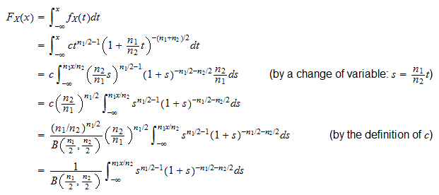
The cumulative distribution function is

${\displaystyle F(x;d_{1},d_{2})=I_{d_{1}x/(d_{1}x d_{2})}\left({\tfrac {d_{1}}{2}},{\tfrac {d_{2}}{2}}\right),}$

where I is the regularized incomplete beta function.

Properties

The expectation, variance, and other details about the F(d₁, d₂) are given in the sidebox; for d₂ > 8, the excess kurtosis is

${\displaystyle \gamma _{2}=12{\frac {d_{1}(5d_{2}-22)(d_{1} d_{2}-2) (d_{2}-4)(d_{2}-2)^{2}}{d_{1}(d_{2}-6)(d_{2}-8)(d_{1} d_{2}-2)}}.}$

The k-th moment of an F(d₁, d₂) distribution exists and is finite only when 2k < d₂ and it is equal to

${\displaystyle \mu _{X}(k)=\left({\frac {d_{2}}{d_{1}}}\right)^{k}{\frac {\Gamma \left({\tfrac {d_{1}}{2}} k\right)}{\Gamma \left({\tfrac {d_{1}}{2}}\right)}}{\frac {\Gamma \left({\tfrac {d_{2}}{2}}-k\right)}{\Gamma \left({\tfrac {d_{2}}{2}}\right)}}.}$

The F-distribution is a particular parametrization of the beta prime distribution, which is also called the beta distribution of the second kind.

The characteristic function is listed incorrectly in many standard references (e.g.,). The correct expression is

${\displaystyle \varphi _{d_{1},d_{2}}^{F}(s)={\frac {\Gamma \left({\frac {d_{1} d_{2}}{2}}\right)}{\Gamma \left({\tfrac {d_{2}}{2}}\right)}}U\!\left({\frac {d_{1}}{2}},1-{\frac {d_{2}}{2}},-{\frac {d_{2}}{d_{1}}}\imath s\right)}$

where U(a, b, z) is the confluent hypergeometric function of the second kind.

Related distributions

Relation to the chi-squared distribution

In instances where the F-distribution is used, for example in the analysis of variance, independence of ${\displaystyle U_{1}}$ and ${\displaystyle U_{2}}$ (defined above) might be demonstrated by applying Cochran's theorem.

Equivalently, since the chi-squared distribution is the sum of squares of independent standard normal random variables, the random variable of the F-distribution may also be written

${\displaystyle X={\frac {s_{1}^{2}}{\sigma _{1}^{2}}}\div {\frac {s_{2}^{2}}{\sigma _{2}^{2}}},}$

where ${\displaystyle s_{1}^{2}={\frac {S_{1}^{2}}{d_{1}}}}$ and ${\displaystyle s_{2}^{2}={\frac {S_{2}^{2}}{d_{2}}}}$, ${\displaystyle S_{1}^{2}}$ is the sum of squares of ${\displaystyle d_{1}}$ random variables from normal distribution ${\displaystyle N(0,\sigma _{1}^{2})}$ and ${\displaystyle S_{2}^{2}}$ is the sum of squares of ${\displaystyle d_{2}}$ random variables from normal distribution ${\displaystyle N(0,\sigma _{2}^{2})}$.

In a frequentist context, a scaled F-distribution therefore gives the probability ${\displaystyle p(s_{1}^{2}/s_{2}^{2}\mid \sigma _{1}^{2},\sigma _{2}^{2})}$, with the F-distribution itself, without any scaling, applying where ${\displaystyle \sigma _{1}^{2}}$ is being taken equal to ${\displaystyle \sigma _{2}^{2}}$. This is the context in which the F-distribution most generally appears in F-tests: where the null hypothesis is that two independent normal variances are equal, and the observed sums of some appropriately selected squares are then examined to see whether their ratio is significantly incompatible with this null hypothesis.

The quantity ${\displaystyle X}$ has the same distribution in Bayesian statistics, if an uninformative rescaling-invariant Jeffreys prior is taken for the prior probabilities of ${\displaystyle \sigma _{1}^{2}}$ and ${\displaystyle \sigma _{2}^{2}}$. In this context, a scaled F-distribution thus gives the posterior probability ${\displaystyle p(\sigma _{2}^{2}/\sigma _{1}^{2}\mid s_{1}^{2},s_{2}^{2})}$, where the observed sums ${\displaystyle s_{1}^{2}}$ and ${\displaystyle s_{2}^{2}}$ are now taken as known.

In general

• If ${\displaystyle X\sim \chi _{d_{1}}^{2}}$ and ${\displaystyle Y\sim \chi _{d_{2}}^{2}}$ (Chi squared distribution) are independent, then ${\displaystyle {\frac {X/d_{1}}{Y/d_{2}}}\sim \mathrm {F} (d_{1},d_{2})}$
• If ${\displaystyle X_{k}\sim \Gamma (\alpha _{k},\beta _{k})\,}$ (Gamma distribution) are independent, then ${\displaystyle {\frac {\alpha _{2}\beta _{1}X_{1}}{\alpha _{1}\beta _{2}X_{2}}}\sim \mathrm {F} (2\alpha _{1},2\alpha _{2})}$
• If ${\displaystyle X\sim \operatorname {Beta} (d_{1}/2,d_{2}/2)}$ (Beta distribution) then ${\displaystyle {\frac {d_{2}X}{d_{1}(1-X)}}\sim \operatorname {F} (d_{1},d_{2})}$
• Equivalently, if ${\displaystyle X\sim F(d_{1},d_{2})}$, then ${\displaystyle {\frac {d_{1}X/d_{2}}{1 d_{1}X/d_{2}}}\sim \operatorname {Beta} (d_{1}/2,d_{2}/2)}$.
• If ${\displaystyle X\sim F(d_{1},d_{2})}$, then ${\displaystyle {\frac {d_{1}}{d_{2}}}X}$ has a beta prime distribution: ${\displaystyle {\frac {d_{1}}{d_{2}}}X\sim \operatorname {\beta ^{\prime }} \left({\tfrac {d_{1}}{2}},{\tfrac {d_{2}}{2}}\right)}$.
• If ${\displaystyle X\sim F(d_{1},d_{2})}$ then ${\displaystyle Y=\lim _{d_{2}\to \infty }d_{1}X}$ has the chi-squared distribution ${\displaystyle \chi _{d_{1}}^{2}}$
• ${\displaystyle F(d_{1},d_{2})}$ is equivalent to the scaled Hotelling's T-squared distribution ${\displaystyle {\frac {d_{2}}{d_{1}(d_{1} d_{2}-1)}}\operatorname {T} ^{2}(d_{1},d_{1} d_{2}-1)}$.
• If ${\displaystyle X\sim F(d_{1},d_{2})}$ then ${\displaystyle X^{-1}\sim F(d_{2},d_{1})}$.
• If ${\displaystyle X\sim t_{(n)}}$ — Student's t-distribution — then: $${\displaystyle {\begin{aligned}X^{2}&\sim \operatorname {F} (1,n)\\X^{-2}&\sim \operatorname {F} (n,1)\end{aligned}}}$$
• F-distribution is a special case of type 6 Pearson distribution
• If ${\displaystyle X}$ and ${\displaystyle Y}$ are independent, with ${\displaystyle X,Y\sim }$ Laplace(μ, b) then $${\displaystyle {\frac {|X-\mu |}{|Y-\mu |}}\sim \operatorname {F} (2,2)}$$
• If ${\displaystyle X\sim F(n,m)}$ then ${\displaystyle {\tfrac {\log {X}}{2}}\sim \operatorname {FisherZ} (n,m)}$ (Fisher's z-distribution)
• The noncentral F-distribution simplifies to the F-distribution if ${\displaystyle \lambda =0}$.
• The doubly noncentral F-distribution simplifies to the F-distribution if ${\displaystyle \lambda _{1}=\lambda _{2}=0}$
• If ${\displaystyle \operatorname {Q} _{X}(p)}$ is the quantile p for ${\displaystyle X\sim F(d_{1},d_{2})}$ and ${\displaystyle \operatorname {Q} _{Y}(1-p)}$ is the quantile ${\displaystyle 1-p}$ for ${\displaystyle Y\sim F(d_{2},d_{1})}$, then $${\displaystyle \operatorname {Q} _{X}(p)={\frac {1}{\operatorname {Q} _{Y}(1-p)}}.}$$
• F-distribution is an instance of ratio distributions
• W-distribution is a unique parametrization of F-distribution.

See also

References

External links

• Table of critical values of the F-distribution
• Earliest Uses of Some of the Words of Mathematics: entry on F-distribution contains a brief history
• Free calculator for F-testing